Machine Learning: Prologue

This post is part of a series of notes on machine learning.

Machine learning is an awful name for a really simple idea.

For me, that name conjures up images of impossibly complex intelligent robots, and it gets worse with terms like “feedforward”, “backpropagation”, “neural network”, and “perceptron”. Combined with the seemingly magical applications of ML, for a long time I assumed it was one of those things I just didn’t have the spare energy to understand.

I finally took the plunge and started getting into the details of machine learning, and it turns out I was wrong. Really wrong! The basic ideas of machine learning are very accessible to anyone with exposure to calculus. Finding good data, tuning your model, and optimizing for GPUs are different questions, and more complicated. But to my eye the apparent magic of ML happens not because the main ideas are complex, but rather because they are effective.

Anyway, the simple idea behind (supervised) machine learning is roughly this, in my words:

1. Suppose we have an interesting but unknown function \(F\), and some sample input-output pairs for this function – say some \((x,y)\) with \(F(x) = y\).
2. Pretend that \(F\) can be approximated by a known function \(G_\theta\), which is parameterized by one or more variables \(\theta\).
3. Use calculus to find the values of the \(\theta\) that makes \(G\) agree with our samples as closely as possible. That is, find \(\theta\) so that \(G_\theta(x) \approx y\).
4. Now use \(G_\theta\) to make predictions about the value of \(F\) at new inputs, under the assumption that \(G_\theta(x) \approx F(x)\) for all \(x\).

A slightly more sophisticated view might be that \(F\) is a function from inputs \(x\) to probability distributions, which we observe to get the output \(y\), but that’s not necessary. The thing is, that function \(F\) could do something really useful and (seemingly) complicated, like decide whether a photo includes a human face or whether a credit card transaction is fraudulent. And it turns out this strategy for approximating \(F\) works really well.

Ok – so what \(G_\theta\) look like? It needs to be complicated enough to be able to approximate \(F\), but also simple enough that we can evaluate it and its gradient efficiently. (Incidentally, this kind of sweet spot between complexity and tractibility shows up a lot.) Typically \(G_\theta\) is modeled using a neural network.

A google image search for “neural network” brings up a bunch of pictures like this:

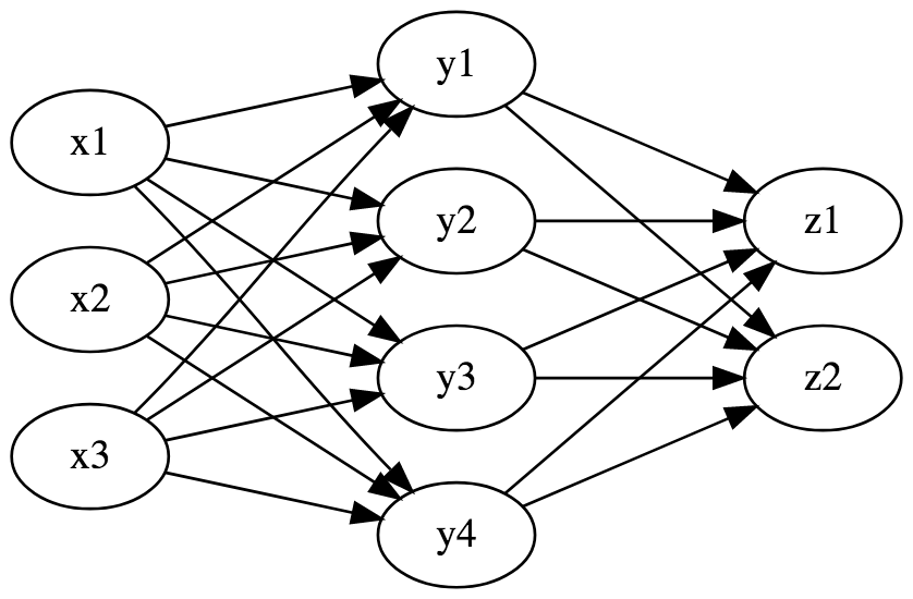
With “weights” and “nodes” in “layers” with “activation functions”. Where’s \(G_\theta\) in this picture? Well, essentially, each column of nodes in that graph represents \(\mathbb{R}^n\) for some \(n\), and the value at each node is a function of the values of the nodes that point to it. So each “layer” in the network is a function with signature \(\mathbb{R}^m \rightarrow \mathbb{R}^n\). In principle that function could be anything, but in practice it’s one of a few different kinds: matrix multiplication, pointwise logistic, and some others. When one layer feeds into the next, we have function composition. Then using the multivariate chain rule it’s possible to compute the gradient of the network in terms of the gradients of each layer.

Maybe some people see diagrams like that and are enlightened. But for me, this way of visualizing neural networks is not helpful at all. For one thing it includes a lot of junk; all those arrows don’t convey very much information. And worse, it obfuscates what the network really is – a function. I’m more comfortable visualizing this as a chain like so. \[\mathbb{R}^3 \stackrel{\psi}{\rightarrow} \mathbb{R}^4 \stackrel{\phi}{\rightarrow} \mathbb{R}^2\] Lo and behold, this is a diagram, representing ordinary function composition, where each arrow takes an extra parameter. Then \(G\) is the composite of these arrows, and \(\theta\) is the direct sum of the parameters at each layer.

To see how far this point of view can go, in this series of posts we’ll develop a crude algebra of neural networks. We’d like to think of a network as a function, and to build complex networks out of simpler ones with (almost) ordinary function composition. I’m mainly interested here in understanding the math, so efficiency will take a backseat. But these posts are literate Haskell and include unit tests; to follow along you can clone this directory from the repo on github and load it into GHCi.